page 36, lines -9 to -5: This calculation of probabilities from a Poisson distribution is in
error, and although the principle of the
example may be correct in some instances, this is not
one of them. Here the incidence of homicide is far greater than Poisson
statistics could
allow, and the ensuing argument makes no sense. Our apologies to the several individuals (and
maybe others)
who asked how the results were calculated and who wasted valuable time trying
to reproduce our erroneous answer.
page 86, line16: It is strongly suggested ....
pages 325, 329: Some of the figures in tables of Appendix B carry more significant figures than they should.
Tables B.5 and B.9
are particularly guilty. Our print formatting led to this error.
Discussions and Clarifications
A. The Anderson-Darling test vs the Kolmogorov-Smirnov test
Both test if the difference between distributions is significant. Both are applicable to
very small samples.
However the A-D test is now accepted as being markedly better
than the K-S Test in most circumstances.
In particular the A-D test is significantly more sensitive to what is happening in the
tails of distributions.
The A-D test is very little more complicated to perform than the K-S (renowned for simplicity!):
1.We have data {Y1,Y2, ....Y
n}, and we put these in order.
2. f is the function against which we are testing the distribution of
Yi, and F is its integral, its
Cumulative Distribution Function (CDF). We are testing if Y could be drawn from f.
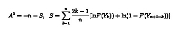
3. Our test statistic is A, calculated from
Compare A against critical values, given the number of
objects in the sample, using tables readily available.
In particular the A-D test is significantly more sensitive to what is happening in the tails of distributions.
The A-D test is very little more complicated to perform than the K-S (renowned for simplicity!):
1.We have data {Y1,Y2, ....Y
n}, and we put these in order.
Compare A against critical values, given the number of
objects in the sample, using tables readily available.
2. f is the function against which we are testing the distribution of
Yi, and F is its integral, its
Cumulative Distribution Function (CDF). We are testing if Y could be drawn from f.
3. Our test statistic is A, calculated from
See http://src.alionscience.com/pdf/A_DTest.pdf
http://cran.r-project.org/web/packages/nortest/nortest.pdf
http://en.wikipedia.org/wiki/Anderson%E2%80%93Darling_test
B. Histogram widths and class intervals
We have emphasized that in general, data binning is bad. It loses
information. Nevertheless as a first step
in data analysis, it is
frequently invaluable, while the use of non-Bayesian methods (if you must), both
parametric and non-parametric, may rely on histogram form.
Missing from both first and second editions of Practical Statistics for Astronomers
is any discussion of
how to histogram data - i.e. bin sizing or class sizing.
We can remedy this by pointing to a Wikepedia
article on The Histogram, providing many references:
http://en.wikipedia.org/wiki/Histogram
There is a summary of methods and prescriptions for bin numbers
and sizes. It's a substantial selection,
including the square-root choice, Sturges' formula, the Rice rule, Doane's formula,
Scott's
normal reference rule, and the Freedman-Diaconis choice. While it may not be clear quite
why so
much work has been expended on this issue, bear in mind how much of medical research
remains
wedded to classical statistical methods, p-values, etc.
The aspect of information loss is not mentioned for the most part. It should always be
remembered
that the more the data has been "histogrammed", the greater the
information-loss, loss of resolution
in particular. Think in terms of pixellated
images, large, low-noise pixels vs small, higher-noise
pixels.
Acknowledgements
While many individuals have sent comments,
we'd particularly like to thank Prof Heinz
Andernach, Universidad de Guanajuato, Mexico for his extensive and helpful
contributions.
how to histogram data - i.e. bin sizing or class sizing. We can remedy this by pointing to a Wikepedia
article on The Histogram, providing many references:
There is a summary of methods and prescriptions for bin numbers
and sizes. It's a substantial selection,
The aspect of information loss is not mentioned for the most part. It should always be
remembered
While many individuals have sent comments,
we'd particularly like to thank Prof Heinz
including the square-root choice, Sturges' formula, the Rice rule, Doane's formula,
Scott's
normal reference rule, and the Freedman-Diaconis choice. While it may not be clear quite
why so
much work has been expended on this issue, bear in mind how much of medical research
remains
wedded to classical statistical methods, p-values, etc.
that the more the data has been "histogrammed", the greater the
information-loss, loss of resolution
in particular. Think in terms of pixellated
images, large, low-noise pixels vs small, higher-noise
pixels.
Acknowledgements
Andernach, Universidad de Guanajuato, Mexico for his extensive and helpful
contributions.